In Plato’s Apology, Socrates declares the famous dictum “an unexamined life is not worth living.” If, instead of establishing Western philosophy, Socrates had decided to become a marketing executive for Athens’ top toga retailer, his quote may well have been “an unexamined lifetime value is not worth… valuing.” Or something like that.

Indeed, predicting customer lifetime value (CLV) has been the cornerstone of modern marketing analytics since the turn of the (third) millennium. It allows marketers to prioritize customers that have the highest predicted business value, and save marketing dollars on those that are unlikely to engage with their brand. Marketers across several industries have used CLV modeling to measure the impact of marketing campaigns, optimize acquisition dollars, and leverage the Pareto principle to maximize the value of their top customers.

Would you rather be the founder of Western philosophy or modern marketing analytics?

The most popular data science approach to predicting CLV is the extended Pareto/NBD model (EP/NBD), which takes as input the classic “RFM” summary statistics from customer transactions: time since most recent purchase (“R”), frequency of repeat purchases (“F”), historical average order value (“M”), and total customer age (which, for some reason, doesn’t get to be part of the acronym). Despite using only a few signals, the EP/NBD model has maintained strong relative performance according to a recent comparison of several CLV prediction approaches.

There have been several attempts to improve CLV prediction via modern machine learning techniques such as SVMs, boosted decision trees, and neural networks, but these models also rely on the time-series of past customer transactions as the primary data signal. We at Amperity believe that further improvements to CLV prediction, and predictive analytics in general, are more likely to come from exploiting new sources of customer data rather than modeling techniques or feature engineering. To quote Rule #41 from Google’s Rule of Machine Learning: “When performance plateaus, look for qualitatively new sources of information to add rather than refining existing signals.”

Fortunately, following Rule #41 has never been easier, since modern businesses collect more types of data about their customers and marketing interactions than ever before. The diversity of data sources has grown so significantly that many retailers and other direct-to-consumer businesses now rely on dedicated customer data platforms (CDPs), like Amperity, to unify this data. Intuitively, these data sources can improve prediction quality in many ways. Customers who purchase a specific product may be more likely to churn. Customers living close to a high-performing store might have higher long-term value. A customer who hasn’t purchased in a while, but who clicks on a marketing email and spends time browsing a catalogue, may be less likely to churn than their unclicking, unbrowsing counterpart.

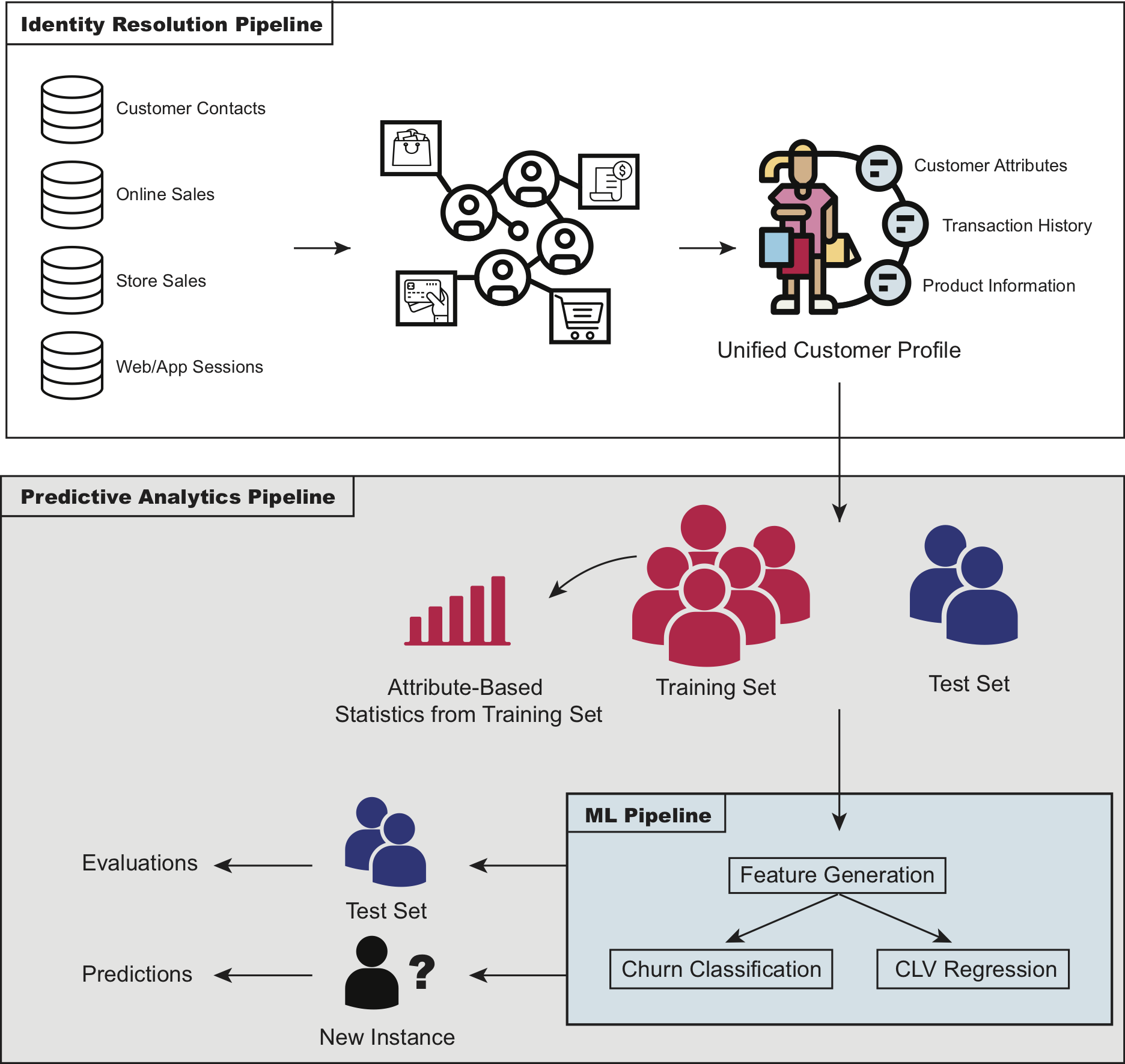High-level overview of the CLV framework

Training on Unified Customer Data

One of the consequences of collecting customer data across multiple channels is that events associated with a given customer may be split across different records with no primary key to connect them. This identity resolution failure has many important consequences, but one of them is that it compromises the quality of predictive analytics. If you’re predicting future spend for individual customers but your historical information is inaccurate, this will undoubtedly impact the quality of the predictions. Based on a sample of real-world data from some of Amperity’s retail customers, we found that before identity resolution 53% of total historical CLV spend was attributed to the wrong customer.

A New Approach to Modeling CLV and Churn

Our data science team has spent the last several months developing a state-of-the-art CLV and churn prediction pipeline that amplifies the value of unified customer data by extending the data that can be used in a CLV model. The approach we settled on is simple: use modeling techniques that put as much explanatory power in the hands of customer data as possible. This, along with every data scientist’s favorite razor related mantra, led us to choose the age-old approaches of linear regression for CLV, and logistic regression for churn.

Specifically, we created an ensemble model that consists of three regression-based variants.

1. A linear regression that directly fits on historical CLV over horizon \(\Delta t\):

   \[\text{CLV}_{1, \Delta t} = w_1^T x + b_1\]

   where \(x\) is a vector of features and \(w\) and \(b\) are length-\(M\) vectors of coefficients and intercepts, respectively.

2. A model that decomposes CLV into two separate predictions, one for churn and one for the CLV of non-churned customers. First a logistic regression is trained on the binary outcome of whether a customer returned over the horizon \(\Delta t\), and then a linear regression is trained on returned customers’ spend in \(\Delta t\):

   \[\begin{aligned} &\text{P}(\text{return}_{\Delta t}) = \frac{1}{1 + e^{(w_2^T x + b_2)}} \\ &\text{CLV}_{2, \Delta t} = \text{P}(\text{return}_{\Delta t}) \cdot \left(w_3^T x_{\text{returned}} + b_3\right) \\ \end{aligned}\]

   Note that we use the same feature vector \(x\) for both churn and CLV, but we estimate different coefficients and intercepts.

3. A model that further decomposes Approach 2 by splitting CLV for non-churned customers into two linear regressions, one on the number of transactions placed by returned customers in \(\Delta t\) (\(\text{orders}_{\text{returned},\Delta t}\)), and one on the average spend by returned customers in \(\Delta t\) (\(\bar{\text{spend}}_{\text{returned},\Delta t}\)):

   \[\begin{aligned} &\text{orders}_{\text{returned},\Delta t} = w_4^T x_{\text{returned}} + b_4 \\ &\bar{\text{spend}}_{\text{returned},\Delta t} = w_5^T x_{\text{returned}} + b_5 \\ &\text{CLV}_{3, \Delta t} = \text{P}(\text{return}_{\Delta t}) \cdot \text{orders}_{\text{returned},\Delta t} \cdot \bar{\text{spend}}_{\text{returned},\Delta t} \\ \end{aligned}\]

   Where \(\text{P}(\text{return}_{\Delta t})\) is the same as in Approach 2.

Our final model is a simple ensemble of these three variants that uses the best performer according to an in-sample validation over \(\Delta t\):

In other words, if we’re predicting CLV and churn at time \(T\) over horizon \(\Delta t\), then we’ll first fit the model at time \(T - \Delta t\), evaluate performance over \(\Delta t\) from that point, then use the best performing variant for our model at \(T\).

Lots and lots (and lots) of features

Crucially, our approach is able to leverage unified customer datasets to incorporate features that have historically been missing from CLV models. Given our relatively simple modeling technique, much of our time was spent creating a robust and stable infrastructure that can handle a vast amount of input data. There are four broad categories of features we explored:

• Customer Attributes: Both raw and engineered features based on demographic information and non-transactional customer behavior such as age, nearest store location, credit card enrollment, and loyalty status.
• Product Attributes: When available, information on the products that customers have purchased, such as most common product category, as well as engineered features such as the proportion of customers that purchased a given category and made a repeat purchase in the subsequent period.
• Transaction Attributes: Broadly similar to the inputs EP/NBD uses; frequency and recency of transactions, as well as average historical spend. We also include data points the EP/NBD is unable to use, such as last order channel and most common order medium.
• EP/NBD Predictions: Predictions from a popular baseline to understand how much marginal value is given by the preceding feature groups.

Since many of these features are correlated, we apply L2 regularization to each of the regression variants above to ensure that our ensemble has stable coefficient estimates and predictions.

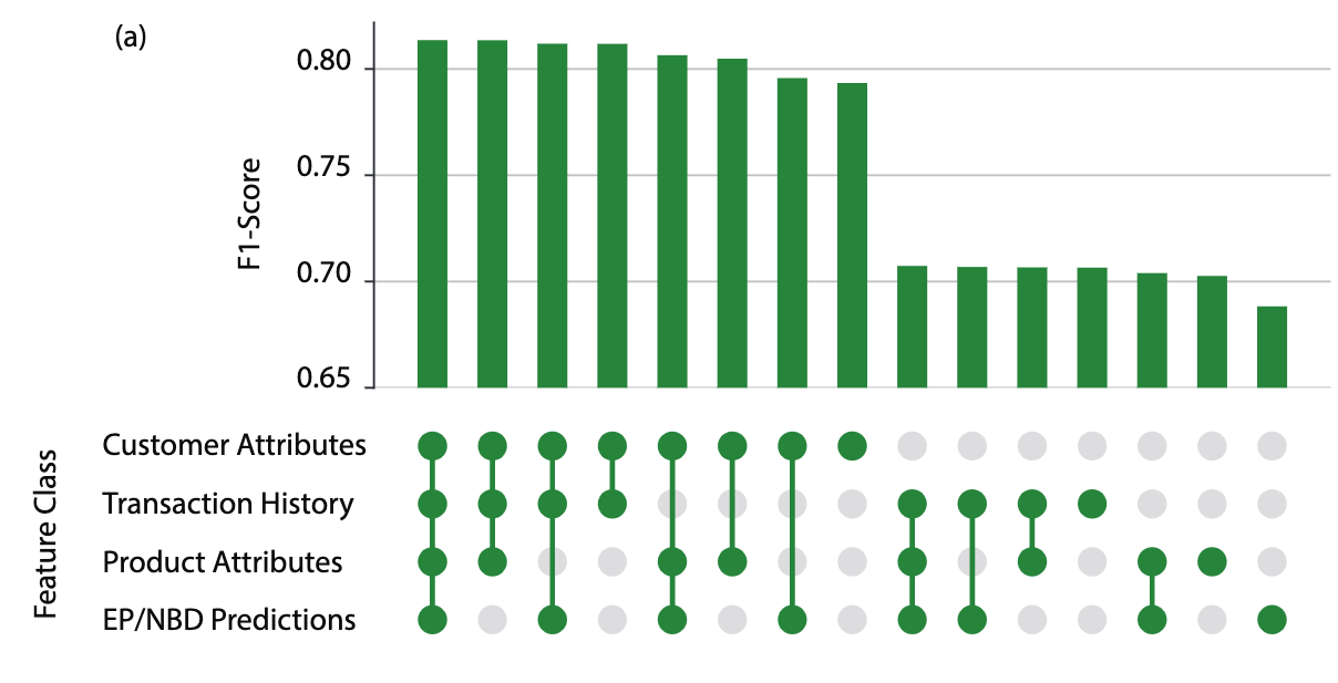A feature ablation study on churn F1 score performed on one of the retailers

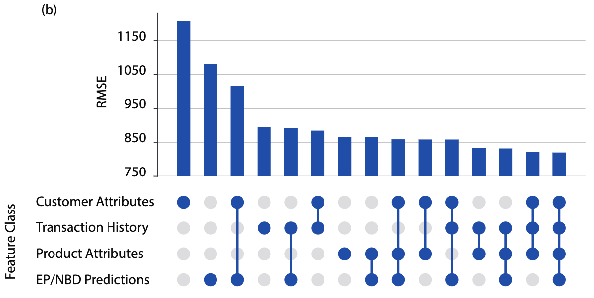A feature ablation study on CLV RMSE performed on one of the retailers

So how’d it do?

In practice, marketers are usually interested in CLV and churn predictions over a small set of future horizons, such as 30, 90, or 365 days. A shorter horizon may be used for win-back or clearance campaigns, whereas a longer horizon is suitable for things like loyalty program and credit card signup outreach. Marketers also tend to leverage CLV using two different prediction modes: Either predictions are made at the same point in time for all customers (“fixed-date” mode), or right after each purchase event (“post-purchase” mode). Traditional CLV analyses have used fixed-date mode, which can be helpful for building out a schedule of marketing campaigns or regularly evaluating business health. Post-purchase mode, on the other hand, is becoming increasingly relevant as marketers execute personalized customer touchpoints in real time. To the best of our knowledge, this was the first CLV analysis to provide empirical post-purchase mode results.

To incorporate these different use-cases, we focused our empirical study on four different prediction settings, parameterized by the prediction horizon (\(\Delta t\)) in days and prediction mode (\(m\)): (\(\Delta t = 90\), \(m =\) fixed-date), (\(\Delta t = 90\), \(m =\) post-purchase), (\(\Delta t = 365\), \(m =\) fixed-date), (\(\Delta t = 365\), \(m =\) post-purchase).

We evaluated our model on three major retailers that use Amperity, using the EP/NBD as a baseline. Compared to the EP/NBD, across the three retailers and four prediction settings, our ensemble improved CLV RMSE by 15.2% and churn F1 score by 13.4% on average. Our model outperformed the baseline by the widest margin in the (\(\Delta t = 365\), \(m =\) fixed-date) setting (\(\approx\) 30%), though we saw improvements in RMSE and F1 score in each of the four settings.

What’s next?

As Amperity continues to develop a state-of-the-art 360° customer view, we’re incredibly driven to refine our modeling techniques and data infrastructure. Some things we’re thinking about:

• Automated feature selection: While regularization techniques allow us to throw as many features into the model as we want, this is often computationally infeasible. We envision a pre-processing step that runs a time-series cross validation on different subsets of features in parallel and returns the optimal set for predicting in the wild.

• More data sources: While our paper included more features than any other CLV and churn analysis to date, there’s always room for more. For example, we would love to generate features from clickstream data and customer-touchpoint (i.e. marketing outreach) data.

• Cutting edge modeling techniques: While our regression-based ensemble performed well in this analysis, and allowed us to incorporate hundreds of features while maintaining a modest runtime, we feel that with infrastructural improvements we could deploy modern ML techniques such as boosted decision trees and neural networks. Such approaches would extract even more value, both predictive and explanatory, from our rich set of features.

If that examination of lifetime value wasn’t thorough enough for you, good! Make Socrates proud and read through our predictive CLV paper for a full download of CLV wisdom, togas sold separately.